R Plotly Draw Map in 3d Plane
How to Create 2D and 3D Interactive Weather Maps in Python and R
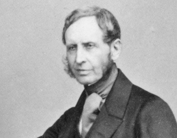
Information technology was the year 1860. Robert FitzRoy, of England and New Zealand, was using the new telegraph organisation to gather daily weather observations and produce the first synoptic weather map. He coined the term "weather forecast" and his were the first always to be published daily.
Fitzroy probably would have never imagined in his wildest dreams what the atmospheric condition map scene would be like 160 years into the future…
⏩ ⏩ ⏩
In 2018, weather maps are commonly produced in the Grid Analysis and Display System (GrADS), R, and Python.
Weather condition and climate maps in Plotly add a new layer to the interrogation of our atmosphere. When information technology comes to these maps, Plotly's point of difference comes in its ability to hover-over and interact with specific data points on the fly, instead of looking at a legend and 'ballparking' a value.
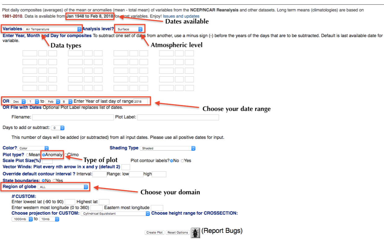
Below, you'll detect several new examples of weather and climate maps created from freely available data on the web. If you'd like to create similar maps, you'll have to get familiar with the NCEP Reanalysis plotter, an amazingly useful tool that is used to investigative the climate system and day-to-day weather.
Here's a short tutorial:
Go alee, immerse yourself in this new and amazing interactive weather earth that we are so fortunate to have in 2018.
Temperature Bibelot
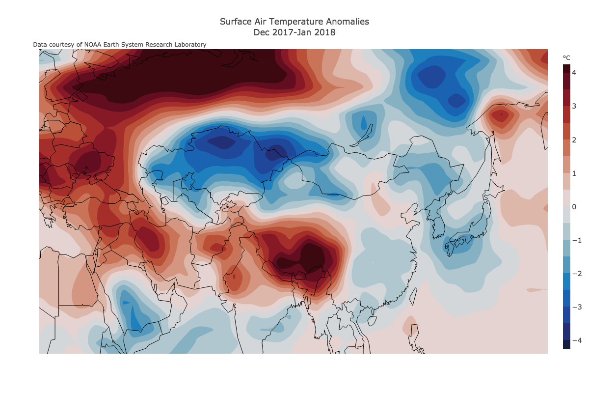
Do you live in the eastern Northward America? If and so, you've were subject to some of the coldest temperatures (with respect to normal) on the globe during December and Jan 2018. Siberia, a place that is already brutally cold during winter, was also colder than average.
On the flip side, the Arctic (wintertime), Europe (winter), eastern Commonwealth of australia (summer), and New Zealand (summer) take had higher up average temperatures during Dec-Jan. In fact, Jan was New Zealand'southward warmest calendar month of whatsoever month on record (nationwide records began in 1909).
See the blue patch to the westward of South America? That'due south associated with a climate signature known as La Niña, defined by libation that normal body of water temperatures in that part of the globe that has wide-reaching impacts on a global scale.
Temperature Difference from Normal 🌡️
Information source: NCEP Reanalysis Plotter.
Data used to create this plot: GitHub.
Python lawmaking: Jupyter notebook.
R code: Make this in R.
Rainfall Bibelot 🌧️
Nosotros tin utilise the same techniques that we used to create the temperature anomaly map to a higher place to atmospheric precipitation (rain and snow).
The map beneath looks at precipitation as a deviation from normal for the menstruum Dec to January 2018.
The Western Pacific had wetter than normal weather chiefly because of La Niña. La Niña is associated with warmer than boilerplate sea surface temperatures near the Philippines, Papua New Guinea, and across Southeast Asia. These warm seas outcome in more rising move than average in the atmosphere, which culminates in rainy weather condition.
In direct contrast, at that place is quite a bit of brown shading about southern Africa as Cape Town approaches Day Zero. In addition, California sticks out along the West Declension of North America for being a much drier than normal location.
Precipitation Difference from Normal
Data source: NCEP Reanalysis Plotter.
Information used to create this plot: GitHub.
Python lawmaking: Jupyter notebook.
R code: Make this in R.
Zoom
While you can ever zoom in on a global projection, peradventure you're looking for something more localized. In this case, you tin can set your latitude and longitude equally such:
          layout = Layout(
            title=title,
            showlegend=False,
            hovermode="closest",        # highlight closest betoken on hover
            xaxis=XAxis(
            axis_style,
            range=[lon[-185], lon[-105]], # fix your custom longitude
            autorange=Simulated                  ),
              yaxis=YAxis(
              axis_style,
              range=[lat[l], lat[85]], # set your custom latitude
              autorange=False
This the resulting graph volition exist a zoom to Due north America. For farther item, y'all tin add country borders like this:
          # Function generating country lon/lat traces          def get_state_traces():
            poly_paths = m.drawstates().get_paths() # country polygon paths
            N_poly = len(poly_paths)  # use all states
            return polygons_to_traces(poly_paths, N_poly)          # Become listing of of coastline, country, and state lon/lat traces          traces_cc = get_coastline_traces()+get_country_traces()+get_state_traces()
Python code: Jupyter notebook.
Here'south a closer look at southern Africa where Cape Town where the water taps are expected to run dry out on June 4th. After three years of low rainfall and drought or near-drought weather condition, locals and visitors are limited to 50 liters (about thirteen gallons) of h2o per day. For some perspective, the average American uses well-nigh 380 liters per day or almost 8 times the Cape Boondocks restricted corporeality.
Python lawmaking: Jupyter notebook.
Mercator projections, like the graphs above, are popular because they preserve management and are platonic for navigation. They besides have further educational value — such as being a good way of learning the shapes of nations.
However, Mercator maps misrepresent the size of countries and are poorly defined at the poles.
For a different perspective, Plotly user empet mapped the flat Earth onto a sphere for a iii-D experience.
Precipitation Divergence from Normal in iii-D
Sunshine Anomaly 🌞
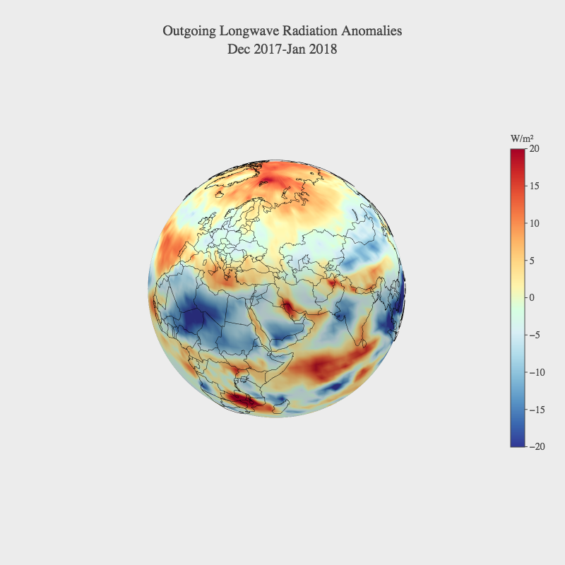
Outgoing longwave radiation (OLR) is a mensurate of the amount of energy emitted to space by world'south surface, oceans and temper. OLR is a practiced proxy for clear skies — the larger (on the positive side) the OLR anomaly, the more unusually articulate it might have been at a given location. Conversely, a large negative bibelot might imply more cloud cover than normal and frequent thunderstorms or rain.
Below, we investigate OLR as a difference from normal for the catamenia December 2017-January 2018.
Above normal sunshine: New Zealand, Queensland, Zimbabwe, Zambia, Portugal, western U.s., Alaska.
Below normal sunshine: Central America, northern Africa, eastern Canada, western Bharat, Philippines and South asia, western Australia.
OLR Divergence from Normal
Information source: NCEP Reanalysis Plotter.
Data used to create this plot: GitHub.
Python code: Jupyter notebook.
R code: Brand this in R.
OLR Difference from Normal in three-D
Python code: Learn how to make this spherical plot.
R code: Make this in R.
Sea Surface Temperature Anomaly
Body of water surface temperatures are the main driver of climate variability in the global tropics (10ºN-10ºS latitude) and play a major role in the global sub-tropics and midlatitudes as well.
Here, nosotros tin identify that a La Niña is present past the 'cool pool' of water plant along the coast of western South America and into the eastern and central equatorial Pacific. La Niña, which is role of the natural El Niño-Southern Oscillation (ENSO) bicycle, is considered to exist a climate driver.
What is not totally natural is the 'carmine blob' between Australia and New Zealand — known as the Tasman Sea marine heatwave. Although this climate feature's evolution was fueled by the ENSO bike, the extent of the anomaly was the largest always observed, near certainly influenced upwards by the tailwind that is anthropogenic global warming.
Data source: NCEP Reanalysis Plotter.
Data used to create this plot: GitHub.
Python code: Jupyter notebook.
R code: Make this in R.
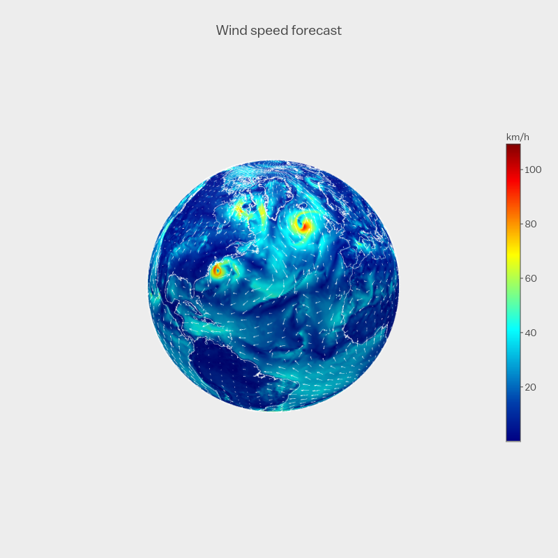
Forecast Wind Speed and Management
The weather goes equally the air current blows. Using weather information in Plotly, not only can you diagnose cyclones, only zoom to low levels to see how much of a breeze is forecast in your town.
The plot below was originally created by Plotly user ToniBois and the 3-D version beneath was created past empet. If y'all wait carefully, y'all'll discover Hurricane Hermine (September 2016) swirling perilously off of the E Coast of the The states.
The data used to create this plot comes from the NCEP Products Inventory.
Colorscales
Looking for the right colorscale to complement your weather map? Look no further: https://react-colorscales.getforge.io/.
The "CMOCEAN" and "DIVERGENT" colorscales are recommended for atmospheric condition and climate charts. For the temperature chart, we used "rest"

For the atmospheric precipitation chart, nosotros used "BrBG"

For the outgoing longwave radiation chart, we used "RdYlBu"
For the body of water surface temperature chart, we used "roll"

Weather and climate maps in Plotly add together a new layer to the interrogation of our atmosphere. When it comes to weather maps, Plotly'southward point of difference comes in its ability to hover-over and interact with specific information points on the fly, instead of looking at a legend and 'ballparking' a value.
Source: https://medium.com/plotly/how-to-create-2d-and-3d-interactive-weather-maps-in-python-and-r-77ddd53cca8
0 Response to "R Plotly Draw Map in 3d Plane"
Post a Comment